Causal Discovery

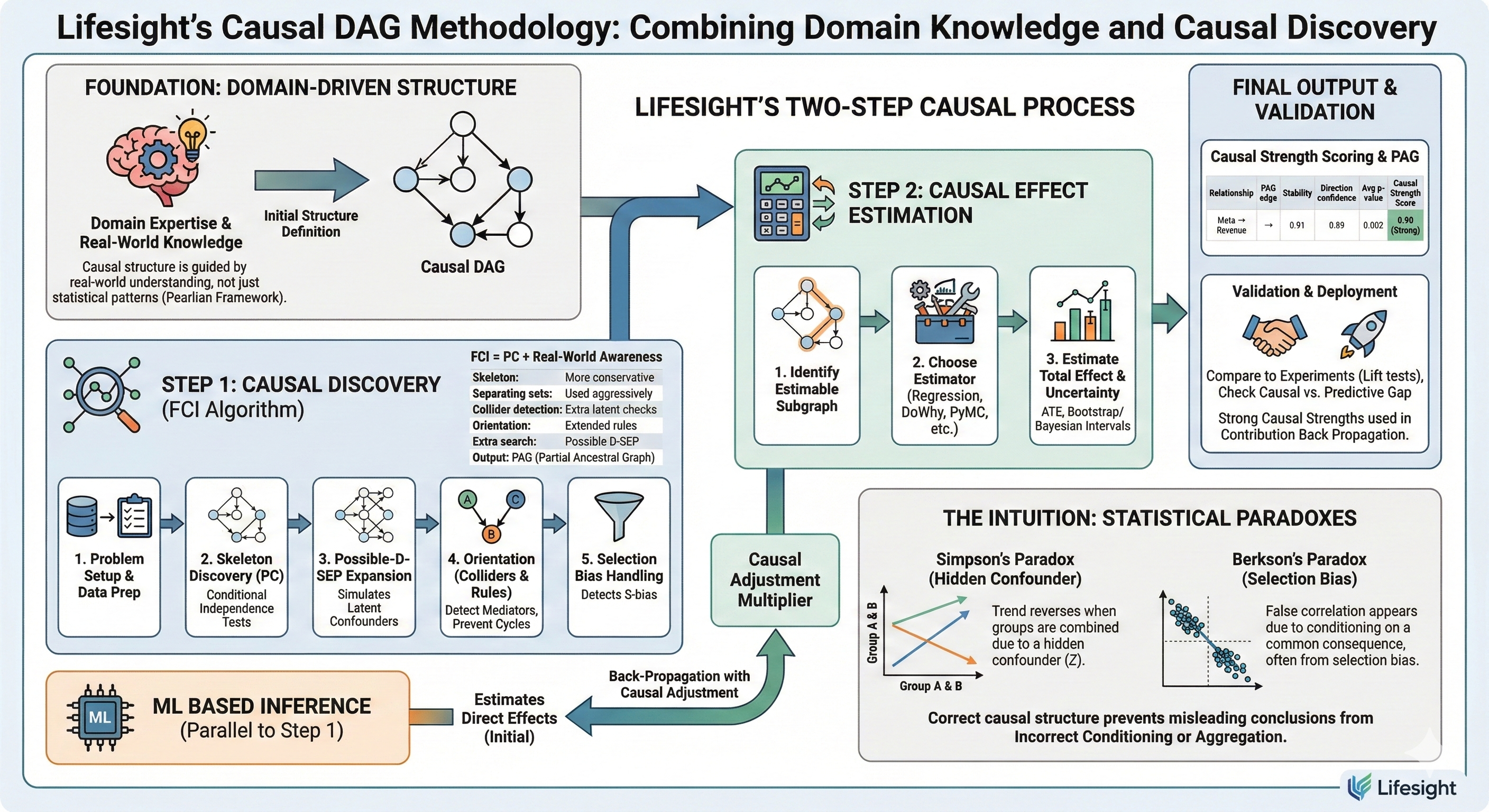
At Lifesight, the structure of the Causal DAG does not start with an algorithm — it starts with deep domain understanding. This principle is also central to the Pearlian framework: causal structure should be guided by real-world knowledge, not just statistical patterns.

Once this initial structure is defined, Lifesight applies a two-step process:

Step 1: Causal Discovery Step 2: Causal Effect Estimation

[Note : ML Based inference, which is the second pillar of MMM framework runs parallel to the Step 1. The Direct effects estimated in this step is then back-propagated using causal adjustment multiplier from Step 2 ]

Statistical Paradoxes and the Intuition behind the need for Causal Graph

Before diving into thee steps of Causal Discovery & Estimation , it is essential to build the right intuition about why causal structure matters in the first place. The fastest way to build this intuition is by understanding two classic causal errors that regularly mislead marketers, analysts, and even advanced models:

Simpson’s Paradox
Berkson’s Paradox

These paradoxes demonstrate how incorrect conditioning or aggregation can completely reverse or fabricate relationships between variables.

Causal Intuition: Simpson’s Paradox vs Berkson’s Paradox

These two paradoxes explain why naïve regression or correlation analysis fails - and why causal graphs are necessary.

Simpson’s Paradox – The Hidden Confounder Problem

Reference 1 - https://brilliant.org/wiki/simpsons-paradox/
Reference 2 - https://en.wikipedia.org/wiki/Simpson%27s_paradox

Simpson's paradox is a phenomenon in probability and statistics in which a trend appears in several groups of data but disappears or reverses when the groups are combined.

Most errors in marketing measurement are not due to weak algorithms, but due to incorrect causal assumptions.

Structure: A hidden variable (Z) influences both X and Y

Fast Causal Inference (FCI) Algorithm

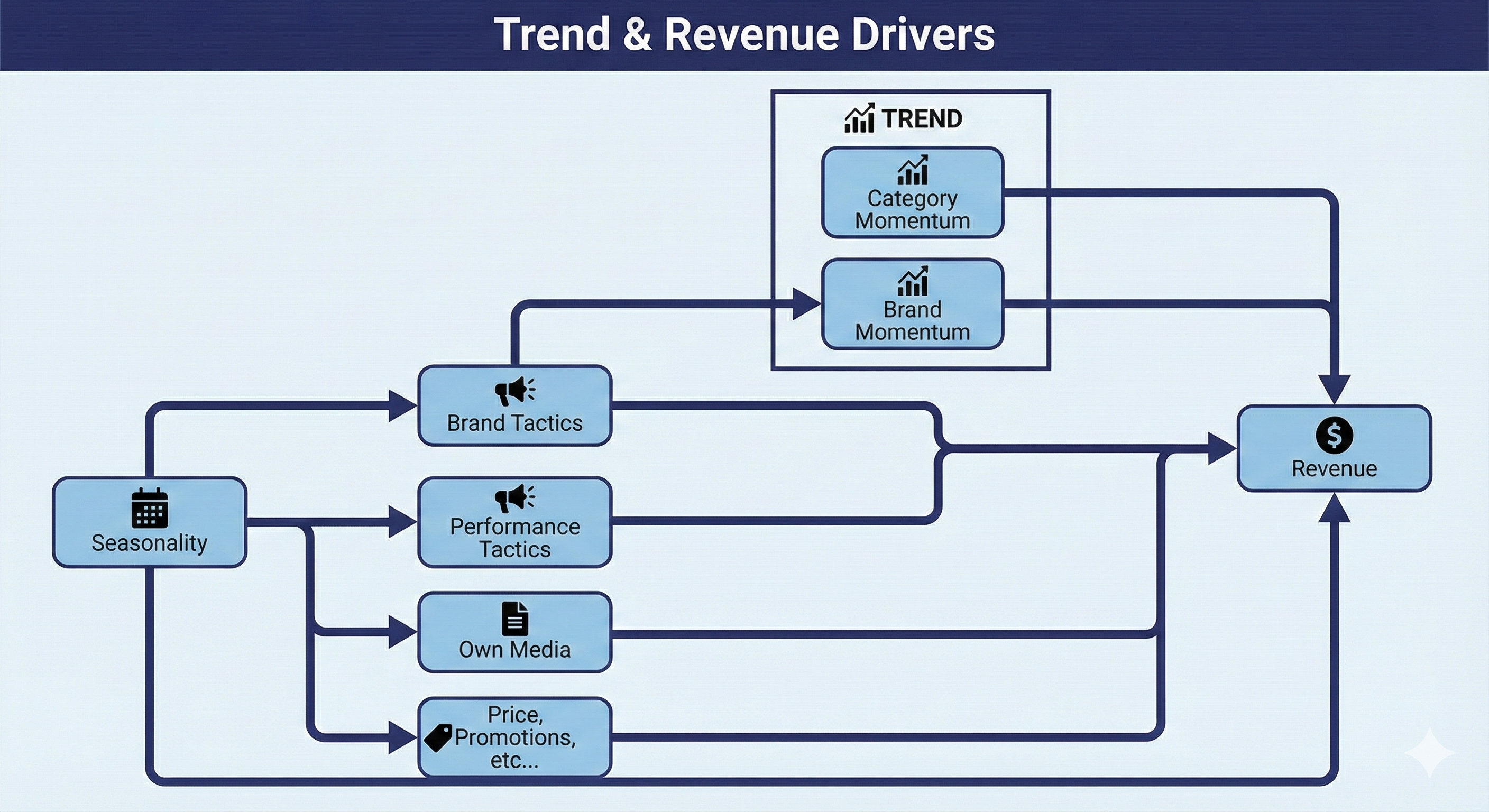
Below mentioned is a broad skeleton of Causal Graph (In the actual causal graph, each of these nodes will be exploded to its specific)

Example : Brand Tactics will be expanded to TV, OOH, Prospecting Tactics across Meta, Google Display, Youtube, TikTok etc... Performance Tactics will be expanded to Search, Retargetting etc...

We then apply the approach know as Fast Causal Inference , which is a very popular variant of PC algorithm, but unlike PC algorithm Fast Causal Inference assumes unobserved variables in the DAG.

FCI = PC + Real-World Awareness

Phase	PC algorithm	FCI algorithm
Skeleton	Uses conditional independence tests to remove edges	Same as PC but more conservative
Separating sets	Stores sepset(A, B)	Same but used later more aggressively
Collider detection	Identifies A → B ← C	Same but with extra latent checks
Orientation	Uses Meek’s orientation rules	Uses extended orientation rules for latent confounders
Extra search	—	✅ Performs additional conditional tests on subsets (Possible D-SEP)
Output	CPDAG	PAG

FCI = PC + extra conditional tests + conservative orientation

FCI Methodology

Phase	Step	What happens (Methodology)	Key Output	What this gives you in MMM / Lifesight
1. Problem setup	1.1 Define variables	Select observed variables (media, revenue, price, seasonality, events, etc.)	Variable set V	Ensures all measurable drivers are accounted
	1.2 Draw prior DAG	Create expert-driven initial DAG (allow partially directed edges)	Prior DAG	Encodes business knowledge & causal beliefs
	1.3 Define constraints	Lock impossible edges (e.g., Revenue → Spend)	Constraint matrix	Prevents nonsensical directions
2. Data prep	2.1 Time alignment	Align all variables to same granularity & lags	Clean dataset	Prevents spurious causal detection
	2.2 Normalization	Scale / transform variables (log, z-score, adstock)	Model-ready data	Improves CI test reliability
	2.3 Stationarity checks	Test for drift / non-stationarity (ADF, KPSS)	Stationary series	Required for accurate inference
3. Skeleton discovery	3.1 Fully connected graph	Start with complete undirected graph	G₀	No assumptions removed yet
	3.2 Cond. independence tests	Remove edges A–B if A ⫫ B	S	Skeleton graph + Sepsets
4. Possible-D-SEP expansion	4.1 Compute Possible-D-SEP	Find nodes that could d-separate A and B with hidden confounders	Expanded conditioning sets	Simulates invisible variables
	4.2 Extra CI tests	Retest adjacencies with PDS	Revised skeleton	Removes false edges missed by PC
5. Orientation (colliders)	5.1 Find v-structures	If A and C not in Sepset with B → mark A → B ← C	Initial directions	Detects mediators
	5.2 Check against PDS	Revalidate with latent-aware logic	Refined v-structures	Avoids false collider claims
6. Orientation (rules)	6.1 Apply extended Meek rules	Orient where logically forced	Directed edges	Prevents cycles
	6.2 Partial orientation	Use ambiguous tails (o→, o-o)	PAG graph	Encodes uncertainty explicitly
7. Selection bias handling	7.1 Detect S-bias	Identify possible selection variables	S-flagged edges	Explains biased correlations
8. Causal strength estimation	8.1 Identify identifiable edges	Keep only directed / semi-directed paths	Estimable subgraph	Safe-to-quantify relationships
	8.2 Choose estimator	Regression / SEM / SCM / DoWhy / PyMC	Estimation engine	Translates structure → effect
	8.3 Estimate total effect	Compute ATE / direct / indirect effects	Effect size	“Spend → Revenue” impact
	8.4 Estimate uncertainty	Bootstrap / MCMC / Bayesian HDI	Confidence / Credible intervals	Model reliability
9. Strength scoring	9.1 Edge stability	Run FCI across subsamples	Stability %	Robustness metric
	9.2 Orientation confidence	% of times same arrow appears	Direction probability	Trust in direction
	9.3 CI test strength	p-value or partial corr	Dependency strength	Relationship reliability
	9.4 Composite causal score	Weighted score: (stability + direction + p)	0–1 causal strength index	Rank channels by causal validity
10. Validation & interpretation	10.1 Compare to experiments	Check aligned with lift tests / geo tests	Coherence score	Ground truth alignment
	10.2 Causal vs predictive gap	Compare vs MMM regression	Divergence measure	Identify overfitting or bias
	10.3 Final decision	Flag strong vs weak assumptions	Causal readiness index	Deployment readiness

Example of the Output

Relationship	PAG edge	Stability	Direction confidence	Avg p-value	Causal Strength Score
Meta → Revenue	→	0.91	0.89	0.002	0.90 (Strong)
TV ↔ Revenue	↔	0.63	0.10	0.04	0.41 (Weak)
Search → Revenue	→	0.95	0.93	0.001	0.94 (Very strong)
Influencer o→ Search	o→	0.55	0.45	0.07	0.50 (Weak)
Email → Revenue	→	0.88	0.90	0.01	0.89 (Strong)

Strong causal strengths are then used in the Contribution Back Propagation approach as mentioned here