In the last few sections we learned about Adstock transformation, Saturation transformation and how we apply evolutionary algorithms to model hyper parameter fine-tuning.

The result of these processes is a set of over hundred thousand , or more, models each of which is a potential solution to your Marketing Mix Problem. We then use advanced AI techniques to search this solution space and pick the solutions that meets multiple criteria of fit

Ranking Methodology

The model selection process starts with a Ranking Method. This ranking method is inspired by the stacking method commonly used in ensemble techniques, where the outputs of multiple base models (level-0) are used as input for a higher-level model (level-1) to enhance predictive accuracy.

We have developed a custom ranking approach that uses Regression Model-based weights. These weights help us rank the models based on several important factors, allowing us to identify the most optimal model for a specific situation.

Key Features Used for Ranking

Our ranking algorithm evaluates models based on several key metrics, including:

nRMSE (Normalized Root Mean Squared Error): Measures the average error between predicted and actual values, normalized to make comparisons easier across models.
Trend: Measures how well the model captures long-term patterns in the data.
Seasonality: Assesses the model's ability to identify recurring patterns, such as weekly or yearly cycles.
Holidays: Captures the effect of irregular events like holidays that can temporarily impact the trends.
Spends (normalized per channel): Reflects the budget allocated to each channel, making them comparable by normalizing the values.
R-squared (Rsq): Shows how well the model explains the variation in the data.
Channel Impact Divergence Index (CDID): A custom metric that measures how much the impact of a particular channel deviates from others in the media mix.

By evaluating models based on these features, we calculate metrics like contribution percentage, ROI (Return on Investment), and error. These metrics help us recommend the most effective solution.

Methodology of Ranking Method Algorithm

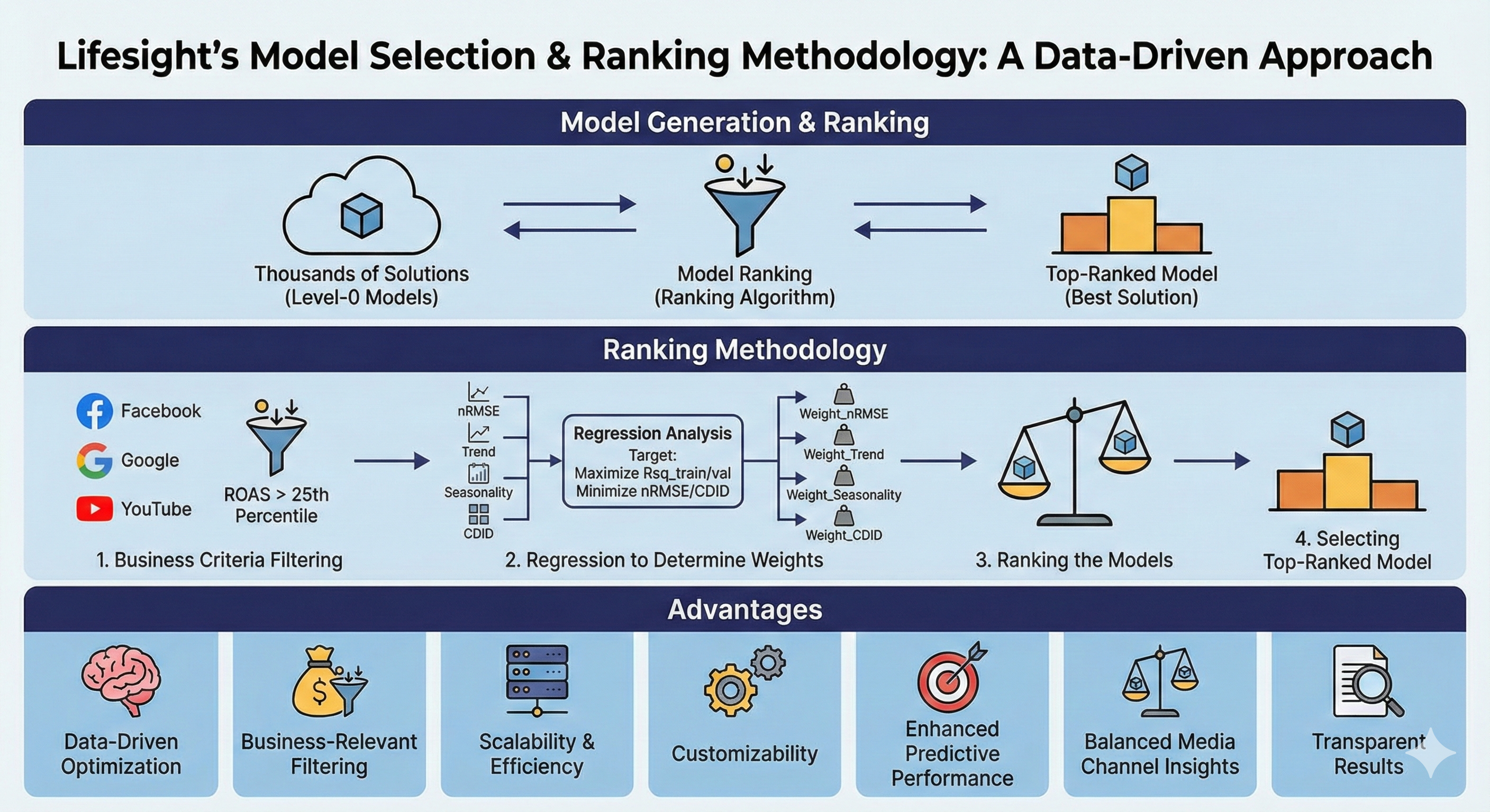
Our ranking method involves a structured process to select the best model. The methodology includes the following steps:

1. Filtering solutions based on business criteria

First, we filter solutions based on a business sense filter. Only solutions with ROAS (Return on Advertising Spend) values higher than the 25th percentile across all media channels are selected for further ranking. This ensures that only high-performing models are considered.

For example, if the 25th percentile for ROAS across Facebook, Google, and YouTube is 1.0, only solIDs with values greater than 1.0 across all three channels are selected.

2. Regression to Determine Weights

To rank the selected solIDs, we perform a regression analysis where the target output is Rsq_train (how well the model fits the training data). The independent variables include the other key metrics such as nRMSE, Trend, Seasonality, and CDID (Channel Impact Divergence Index).

The goal is to maximize Rsq_train and Rsq_val (model accuracy on validation data) while minimizing nRMSE and CDID.
The coefficients derived from this regression are used as weights for each parameter. These weights represent the importance of each feature when evaluating model performance.

3. Ranking the Models

Once we have the weights from the regression analysis, we apply them to the filtered solutions. Each solutions is then scored based on how well it performs across the weighted parameters.

4. Selecting the Top-Ranked Model

After scoring all solutions, the model with the highest score is selected as the top-ranked model. This model is recommended as the most effective solution based on the key business metrics.

Advantages of the Ranking Algorithm

1. Data-Driven Optimization

The ranking algorithm leverages regression-based weighting to ensure that model selection is grounded in objective, data-driven insights. By maximizing key metrics like R-squared (Rsq) while minimizing errors like nRMSE and divergence metrics like CDID, the algorithm identifies the most accurate and reliable models. This ensures that the selected model performs well both on training data and when generalized to unseen data.

2. Business-Relevant Filtering

One of the most impactful features of the algorithm is its ability to filter models using business-relevant metrics, such as ROAS across multiple channels. By applying a business logic filter (e.g., selecting only models with ROAS values above the 25th percentile), the algorithm ensures that only models with real business value and strong ROI potential are considered. This step aligns model selection with financial and strategic goals, making it highly actionable for decision-making.

3. Scalability and Efficiency

The algorithm is built to handle the ranking and analysis of thousands of models efficiently. Its ability to process large-scale data and evaluate numerous solutions ensures that it can be applied to complex datasets without sacrificing performance. This scalability is crucial for businesses that deal with a high volume of models and need rapid, reliable selection processes.

4. Customizability for Specific Use Cases

The ranking methodology is highly customizable, which is essential for adapting the algorithm to specific business scenarios. New features or performance criteria can be easily incorporated, and the weighting of variables can be adjusted to reflect unique industry needs. This ensures that the algorithm can be tailored for different objectives, such as maximizing ROI, improving predictive accuracy, or optimizing media spend.

5. Enhanced Predictive Performance and Model Reliability

By prioritizing models that maximize fit (Rsq) and minimize errors (nRMSE and CDID), the algorithm selects models that provide more accurate predictions and are more reliable in making future forecasts. This reduces the risk of overfitting and ensures that the chosen model performs well in real-world scenarios, leading to better business outcomes and improved decision-making.

6. Balanced Media Channel Insights

The incorporation of the Channel Impact Divergence Index (CDID) ensures that the model's predictions reflect a balanced impact across all media channels. This prevents any one channel from disproportionately influencing the results, which is crucial for optimizing media spend. By identifying the models that fairly allocate contribution across multiple channels, businesses can make more informed and balanced investment decisions.

7. Transparent and Interpretable Results

One of the major strengths of the ranking algorithm is its transparency. The use of regression coefficients as weights for each feature provides clear insight into how each parameter influences the final ranking. This interpretability fosters trust among stakeholders, as they can see exactly why a particular model was chosen, making the decision process more understandable and aligned with business logic.

Confidence Intervals and Uncertainty in ROAS/CPA Calculation

Understanding Bootstrapping

Bootstrapping is a powerful statistical technique to estimate the uncertainty of a metric (like ROAS or CPA) by repeatedly resampling the original data. The basic idea is that by resampling your data, you can generate an empirical distribution of possible outcomes and thereby assess how much your estimate might vary.

Key Concepts of Bootstrapping:

Sampling with Replacement: In bootstrapping, random samples are taken from the original dataset with replacement, meaning that the same observation can be included multiple times in the resampled datasets.
Resampling to Estimate Uncertainty: By repeatedly resampling the dataset, you simulate what it would be like to draw different samples from the population. This allows you to assess how much the estimate might vary if you observed different data.
Standard Error Estimation: Bootstrapping gives a way to compute the standard error of a statistic (such as ROAS or CPA). The standard deviation of the bootstrapped estimates is used as an estimate of the standard error.

Traditional Approach vs. Bootstrap Approach

Traditional Sampling Distribution:

In traditional statistics, you assume that if you could take all possible samples of a given size from a population, the estimates would form a sampling distribution. If the sample size is sufficiently large, the sampling distribution would be approximately normal (bell-shaped), and its standard deviation would be the standard error.

However, when sample sizes are small, or the data doesn’t follow normality, this assumption breaks down, making it difficult to draw reliable conclusions using traditional methods.

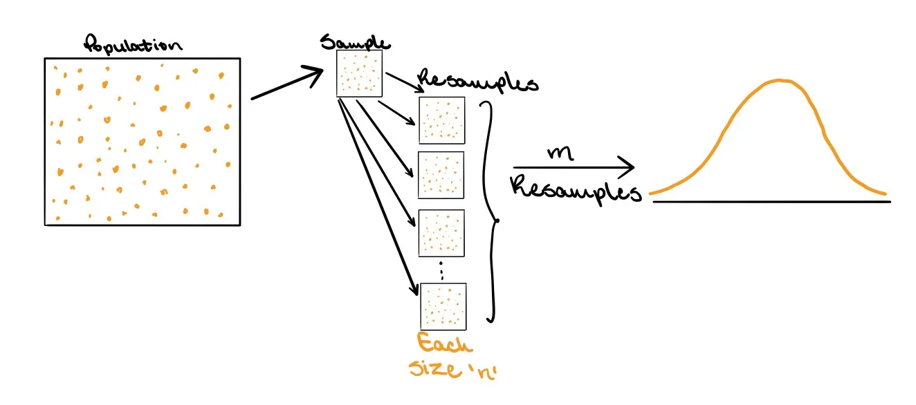
Bootstrapping Approach:

Instead of relying on theoretical distributions, bootstrapping constructs an empirical sampling distribution by:

Drawing a sample of size n from the population.
Resampling from that sample m times with replacement.
Creating a distribution of estimates from these m resampled datasets, which mimics the theoretical distribution.

How Lifesight Implements Bootstrapping:

Lifesight uses bootstrapping to introduce confidence intervals for ROAS and CPA metrics by:

Finding Optimal Models:
- Lifesight calculates optimal models , identifying models that strike the best balance between accuracy and generalizability.
Clustering Models:
- Using clustering techniques such as k-means, Lifesight identifies groups of models with similar hyperparameters. This ensures that each cluster represents a set of models with comparable behavior across channels.
Bootstrap Sampling:
- For each cluster of models and for each channel, Lifesight performs bootstrap resampling on the calculated ROIs.
- From this, Lifesight calculates the confidence intervals and standard error for each channel's ROAS or CPA.

This approach allows for a more robust understanding of how marketing investments perform across channels, offering a deeper level of insight than a single point estimate can provide.

Benefits of Bootstrapping in ROAS/CPA Estimation:

No Distribution Assumption: Unlike traditional methods, bootstrapping doesn’t require the assumption that the data follows a specific distribution (e.g., normal distribution). This makes it applicable to datasets of any size or shape.
Empirical Confidence Intervals: You can directly compute confidence intervals from the resampled data, providing a more accurate estimate of the uncertainty in your ROAS/CPA.
Handling Variability Across Channels: Bootstrapping accounts for variability in channel performance, making the derived ROAS or CPA metrics more reliable and reflective of the true performance.

Conclusion:

Bootstrapping in Lifesight offers a robust way to measure the uncertainty in ROAS or CPA calculations. By resampling the data and calculating empirical confidence intervals, Lifesight provides more reliable estimates, giving users deeper insights into the performance of their marketing channels.

Estimation Error

Estimation error refers to the difference between the actual parameter and the estimated parameter in a model. It is a critical concept in scientific measurements, as it helps assess the accuracy and reliability of results. Since all measurements come with some degree of uncertainty, understanding and accounting for estimation error is essential for improving the precision of predictions and making informed decisions based on data.

Why Is Error Estimation Important?

Error estimation is vital for ensuring the accuracy of any measurement or prediction. By determining the degree of uncertainty in a measurement, we can better understand how reliable our results are. This is especially important in fields that rely on data-driven decisions, where even small errors can lead to incorrect conclusions. Recognizing and addressing these errors is key to improving model performance and the overall quality of data-driven insights.

Types of Estimation Errors

Estimation errors typically fall into three categories:

Bias (Systematic Errors): These occur when the model consistently overestimates or underestimates the true value. Bias is introduced due to incorrect assumptions or faulty measurement techniques and does not cancel out over multiple observations.
Variance (Random Errors): These errors are caused by random fluctuations in the data or measurement process. Unlike bias, variance affects the spread of predictions and tends to average out over time.
Irreducible Error: This is the error inherent in the system that cannot be reduced, no matter how well the model is designed. It arises due to unpredictable variations in the data that cannot be accounted for by the model.

Understanding these three types of estimation errors helps practitioners identify where improvements can be made in model accuracy and prediction reliability.

Sources of Estimation Error

Estimation errors can arise from various factors, including:

Poor Quality or Incomplete Data: Missing data, outliers, and measurement inaccuracies can skew predictions and lead to errors.
Incorrect Assumptions or Model Specifications: Using an inappropriate model (e.g., a linear model for a nonlinear relationship) can introduce bias and result in significant errors.
Small Sample Sizes: Smaller datasets are more susceptible to random variations, which can inflate estimation errors.

How to Quantify Estimation Error

To assess the accuracy of estimates, several commonly used metrics can help measure estimation error, such as:

Mean Absolute Error (MAE):
- MAE measures the average of the absolute differences between predicted and actual values.
- Formula:
  MAE = (1/n) * Σ |Predicted - Actual|
Mean Squared Error (MSE):
- MSE calculates the average of the squared differences between predicted and actual values.
- Formula:
  MSE = (1/n) * Σ (Predicted - Actual)²
Root Mean Squared Error (RMSE):
- RMSE is the square root of the MSE and provides an estimate of the standard deviation of the prediction errors.
- Formula:
  RMSE = √[(1/n) * Σ (Predicted - Actual)²][(1/n) * Σ (Predicted - Actual)²]

📘
At Lifesight, we specifically calculate estimation error using the following formula:

Estimation Error = (Predicted Revenue - Actual Revenue) / Actual Revenue

Reducing Estimation Errors

Both systematic and random errors can be mitigated through careful model design and data handling:

Reducing Systematic Errors:

Model Selection and Validation: Choosing the correct model type and using techniques like cross-validation can help minimize bias introduced by poor assumptions.
Data Cleaning and Preprocessing: Properly handling missing data, outliers, and other anomalies is crucial for reducing systematic error. Ensuring accurate data collection methods also helps avoid bias.
Experiment Design: When designing experiments or collecting data, it's important to avoid known biases (e.g., calibration errors in instruments) and ensure uniformity in how data is gathered.

Reducing Random Errors:

Increase Sample Size: Larger sample sizes help reduce the impact of random noise and make estimates more reliable.
Averaging Multiple Observations: Taking multiple measurements and averaging the results helps reduce the influence of random variations.
Improve Consistency: Ensuring that the same methods and conditions are applied during data collection can help reduce random variability.