Predictive CLTV Modeling

Introduction

Customer Lifetime Value (CLTV) modeling estimates the total value a customer is expected to generate after they are acquired. At Lifesight, predictive CLTV is used to bring forward-looking customer value into measurement and optimization, so that acquisition decisions are made against the value a customer will realize rather than only the cost to acquire them.

This page explains why predictive CLTV is needed, the methodology and underlying statistical logic Lifesight uses, the data required to run it, and how predicted CLTV is used to adjust Incremental CAC (iCAC) and Incremental CPA (iCPA) inside the platform.

The Need for Predictive CLTV

Most ad platforms optimize toward an acquisition event — a signup, a first purchase, an install, a qualified lead. But for many businesses, the conversion that matters is not a single event; value is realized in two steps:

1. Step 1 - Customer Acquisition: the first, trackable conversion (e.g., first order or signup).
2. Step 2 - Value Realization: the value the customer actually generates afterward — typically materializing over 30, 60, 90, or 180 days following acquisition.

When these two steps are separated in time, optimizing on Step 1 alone is misleading:

• A channel can produce cheap acquisitions that realize little downstream value, while another produces more expensive acquisitions that mature into high-value customers. On an acquisition-cost basis the first channel looks better; on a value basis it may be far worse.
• The value of Step 2 is not yet observable at the moment of acquisition. Waiting 30–180 days to learn the true value of today's spend is too slow for daily budget, bid, and creative decisions.

Predictive CLTV solves this by estimating the eventual Step 2 value at (or near) the time of acquisition. This lets the platform optimize acquisition spend toward expected long-term value instead of lowest immediate cost.

📘

When CLTV modeling applies: CLTV modeling is used specifically in two-step conversion businesses — where acquisition and value realization are separated in time. If value is fully realized at the moment of the tracked conversion (single-step), CLTV modeling is not required.

Methodology and Underlying Logic

Lifesight models CLTV using a probabilistic ("buy-till-you-die") framework. Instead of applying flat heuristics (e.g., "average order value × assumed repeat rate"), it models each customer's behavior as a pair of latent random processes and infers the parameters of those processes from observed transaction history.

CLTV is decomposed into two questions that are modeled independently and then combined:

1. How many transactions will this customer make in the future? — modeled by a transaction-frequency / dropout process.
2. How much will each of those transactions be worth? — modeled by a monetary-value process.

The product of the two, projected over a horizon and discounted, yields predicted CLTV.

Inputs: the RFM-T summary

Each customer's raw transaction history is summarized into four quantities:

• Frequency (x): the number of repeat transactions (total transactions minus the first).
• Recency (t_x): the time between the customer's first and last transaction.
• Age (T): the time between the customer's first transaction and the end of the observation window — i.e., how long they have had the opportunity to transact.
• Monetary value (m_x): the average value per (repeat) transaction.

These four numbers per customer are sufficient statistics for the models below — the full event log is not needed once summarized.

Part 1 — Transaction frequency and dropout

The frequency model captures two realities at once: customers transact at different rates, and customers silently become inactive at different points (there is no "cancellation" event — a lapsed customer simply stops). The model is built from four assumptions:

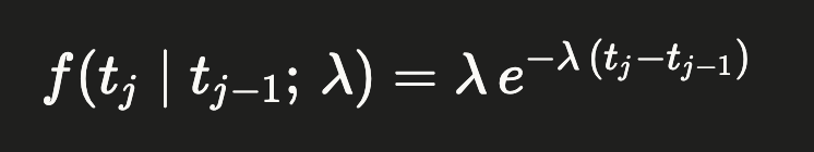
1. While active, a customer transacts as a Poisson process with an individual rate λ. Equivalently, the time between transactions is exponentially distributed:

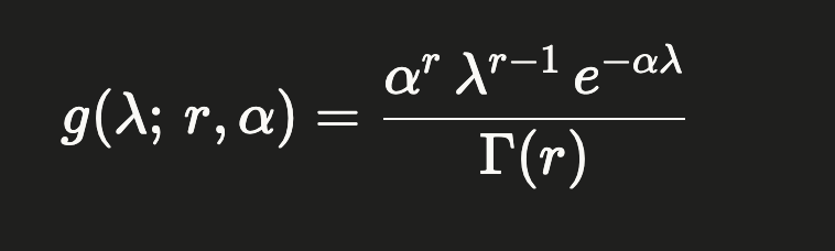
2. Transaction rates differ across customers, with λ drawn from a Gamma distribution. Mixing a Poisson count process over a Gamma-distributed rate yields a Negative Binomial Distribution (NBD) for transaction counts across the population:

3. After each transaction, a customer "drops out" (becomes permanently inactive) with probability p. The number of transactions before dropout is therefore geometrically distributed.
4. Dropout probability differs across customers, with p drawn from a Beta distribution:

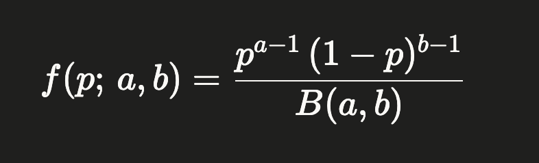
The transaction rate (λ) and dropout propensity (p) are treated as independent across customers. The population-level parameters — r, α (frequency heterogeneity) and a, b (dropout heterogeneity) — are estimated by maximum likelihood over all customers' RFM-T summaries.

From the fitted model, two quantities matter most:

• P(alive): the probability a customer is still active given their recency and age. Intuitively, a customer who used to transact often but has been quiet for a long time relative to their age has a low P(alive); a recently active customer has a high one.
• Expected future transactions: the conditional expectation of the number of transactions a customer will make over a future interval of length t, given their observed frequency (x), recency (t_x), and age (T):

E[ Y(t) | x, t_x, T ]

This closed-form expectation weighs how often the customer has transacted against how likely they are to still be active. (Its full expression involves the Gaussian hypergeometric function; the practical takeaway is that frequent, recently-active customers receive high expected future counts, while frequent-but-lapsed customers are appropriately discounted.)

Part 2 — Monetary value

A separate model predicts the average value of each future transaction. It rests on three assumptions:

The monetary value of a customer's individual transactions varies randomly around that customer's own underlying average.
A customer's average transaction value is stable over time, but differs across customers.
The distribution of average transaction values across customers is independent of how frequently they transact.

Concretely, individual transaction values are modeled as Gamma-distributed around a customer-specific mean, and that mean is itself Gamma-distributed across the population — a Gamma-Gamma structure. The expected average transaction value for a given customer is a credibility-weighted (shrinkage) blend of their own observed average and the population average:

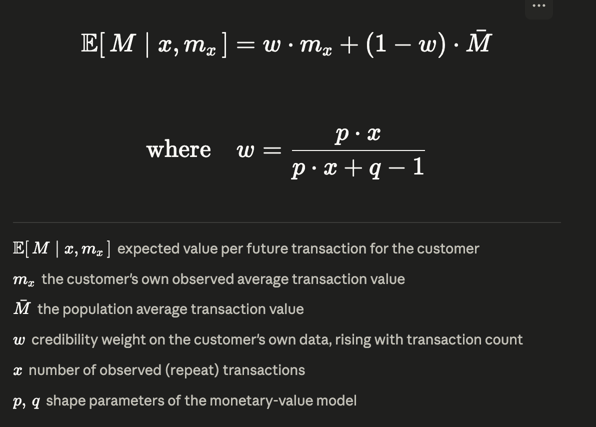
The weight w increases with the number of observed transactions (x). A customer with a long history is trusted mostly on their own average; a customer with few transactions is pulled toward the population mean. This prevents one unusually large or small early order from dominating the estimate.

⚠️ Validation requirement: The monetary model assumes transaction frequency and monetary value are uncorrelated. Before applying it, this independence is checked (e.g., via the correlation between frequency and average value). If a strong correlation exists, the monetary estimates must be treated with caution or segmented.

Combining into CLTV

Predicted CLTV over a horizon is the expected number of future transactions multiplied by the expected value per transaction, summed period-by-period over the horizon and discounted to present value:

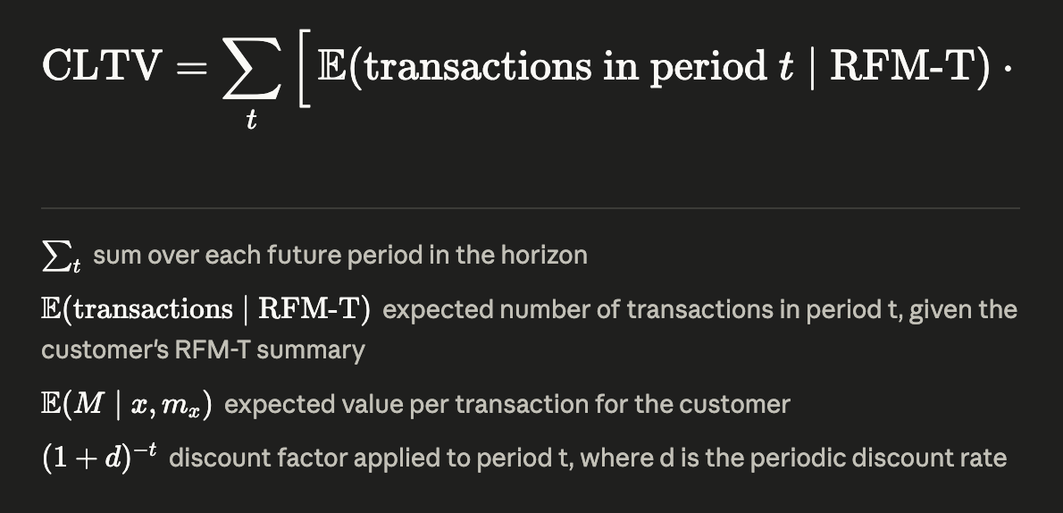
where d is the periodic discount rate and the sum runs across the chosen horizon (e.g., the 30/60/90/180-day windows aligned to value realization). The result is a per-customer expected value that can be aggregated to a cohort or population level.

Summary

Predictive CLTV lets Lifesight act on the value an acquired customer will generate rather than only the cost of acquiring them — essential wherever conversion happens in two steps, with value realized 30–180 days after acquisition. The approach models transaction frequency and dropout as latent probabilistic processes, models monetary value with a credibility-weighted shrinkage estimator, and combines them into a discounted, horizon-bounded value per customer. Run at an aggregate level and adjusted against channel-level iCAC / iCPA, predicted CLTV turns acquisition-cost optimization into long-term-value optimization.